Choices with Consequences #2: Data Processing Decisions in Household Surveys

Posted on August 5, 2026August 4, 2026

Defining “Urban” and “Rural”: How Urban-Rural Boundaries Shape What We Know About Development, especially when “rural” is simply what is not “urban.”

Key Takeaways

Definitions of “rural” and “urban” can affect indicators of economic development used for decision-making and funding allocations.
Within countries, periodically re-categorizing households as rural or urban can affect measures of rural poverty and other welfare indicators.
Across countries, different classifications can vary considerably and limit valid comparisons.

Urban versus Rural Categorization

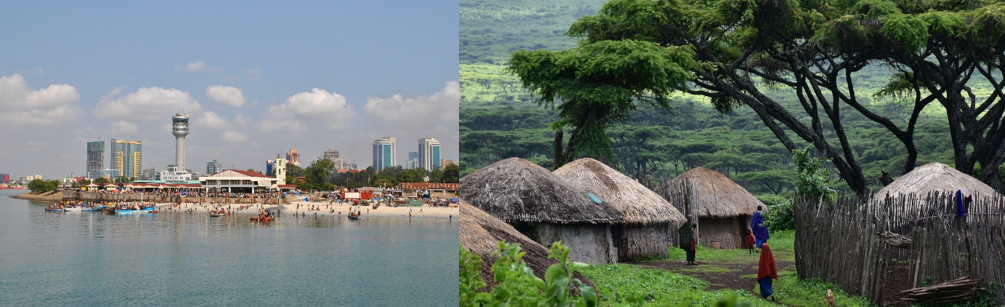
The majority of countries use an administrative definition to distinguish between urban and rural areas based on thresholds of population, density, size, or economic development. But despite urban / rural categorizations commonly being used in agricultural and development analyses, and within global monitoring systems such as the Sustainable Development Goals (SDGs), there is no universal standard.

Almost a decade ago Moreno (2017) noted: Localities in Denmark or Iceland are urban above 200 inhabitants or more, whereas the Netherlands and Nigeria use a threshold of 20,000, Mali 30,000, and Japan 50,000 inhabitants. Some countries use multiple criteria. “For instance, urban areas in Bhutan need to satisfy at least 4 conditions out of 5 criteria: a minimum population (1,500 inhabitants), a threshold in population density (1,000 persons per sq. km), depend on non-primary economic activities (more than 50%), a minimum requirement for the area of the urban center (not less than 1.5 sq. km.), and the need to have economic potential for future growth (revenue base)” (Moreno, 2017, p. 3).

In all countries, urban–rural classifications play a central role in guiding policy interventions and serve as an important stratification variable in data collection. To understand how alternative urban vs. rural categorizations affect development indicators and related policy conclusions, in this blog, we summarize the approach followed in Wineman et. al (2020). We use data from four waves of the nationally representative data from Tanzania and Nigeria, focusing on the Tanzania National Panel Living Standards Measurement Study (TZNPS) from 2008 through 2014 as a case study. This dataset captures rural and urban households based on the country’s administrative definition. We also draw from various secondary data sources such as the 2013 WorldPop data set, 2016 NOAA DMSP-OLS Nighttime Lights Time Series data set, 2017 Global Man-made Impervious (GMIS) data set, 2017 Africapolis data set, and spatial data from Google Earth that have been used across countries and studies to map out urbanization.

Approaches for Defining Urban Areas

Although a country’s administrative definition might be considered the default for measuring “urban” areas, periodic reclassification – usually with a census – that nudges growing rural areas up into the urban category – leaves “rural” as the residual. In many administrative definitions, “Rural” is de facto what is NOT “Urban”. We therefore examine alternative measures of understanding urbanization and rural welfare over time.

		Definition / construction
1.	Administrative definition	The official designation in each country
2.	Population density	A household is categorized as urban if the local population density is at least 500 persons/km²(from WorldPop).
3.	Impervious surface	A household is categorized as urban if the share of impervious surface (man-made surfaces) cover is at least 2% (from the GMIS data set of Landsat).
4.	Night lights intensity	A household is categorized as urban if the intensity of night lights is at least 8 on a scale of 0 to 63 (from the NOAA DMSP-OLS Nighttime Lights Time Series data set).
5.	Africapolis	The designation of urban areas is provided by Africapolis, which bases its determination on the settlement population size (≥ 10,000) and the distance between buildings.
6.	Local economy	A household is categorized as urban if the average share of nonfarm income (excluding crop, livestock, or agricultural wage income) among the nearest 7 neighbors is at least 66%.
7.	Subjective assessment	A household is categorized as urban based on subjective assessment of Google Earth images. This labor-intensive categorization was applied only to the 2014 survey wave.

Table 1. Definitions of “urban” and “rural”

Impacts of Choosing Different Definitions of “Urban”

Cross-country comparisons of urbanization levels are sensitive to definition choice

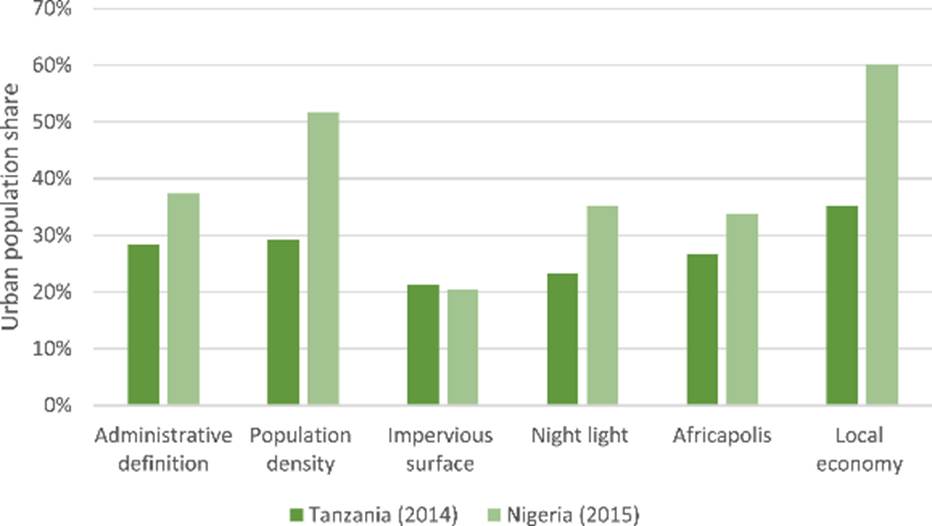
We find that patterns of urbanization levels in Tanzania and Nigeria reverse depending on definition. For example, using the ‘impervious surface’ definition, Tanzania has a slightly larger urban population share than Nigeria. For all other definitions, Tanzania’s urban share is lower than Nigeria.

Figure 1: Cross-country comparison of urbanization levels in Tanzania and Nigeria.

Definition choice swings urbanization levels by ~ 20 percentage points

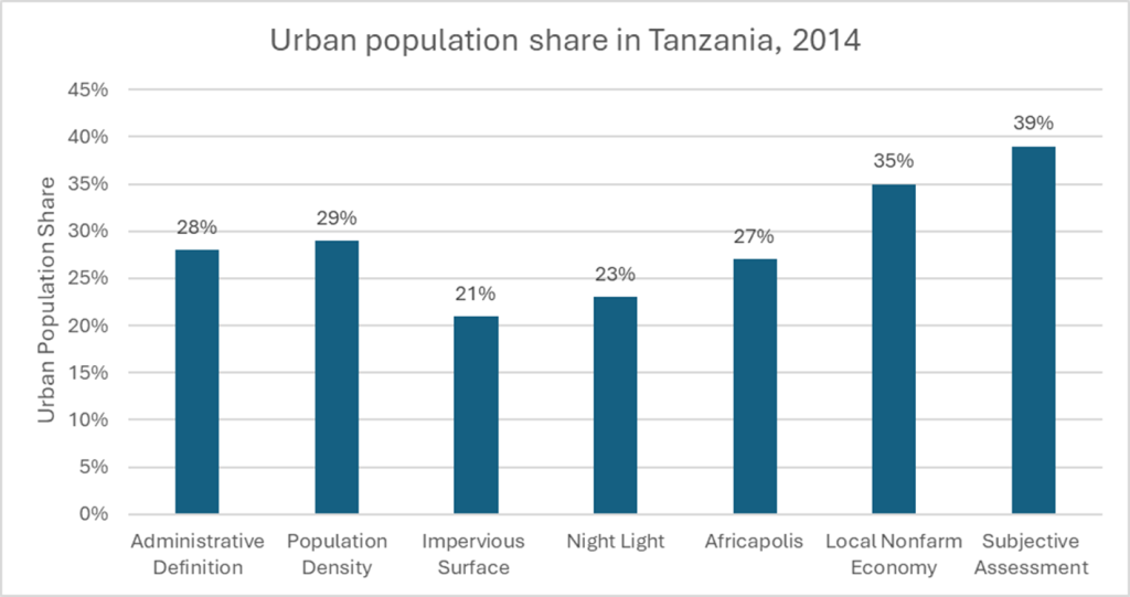
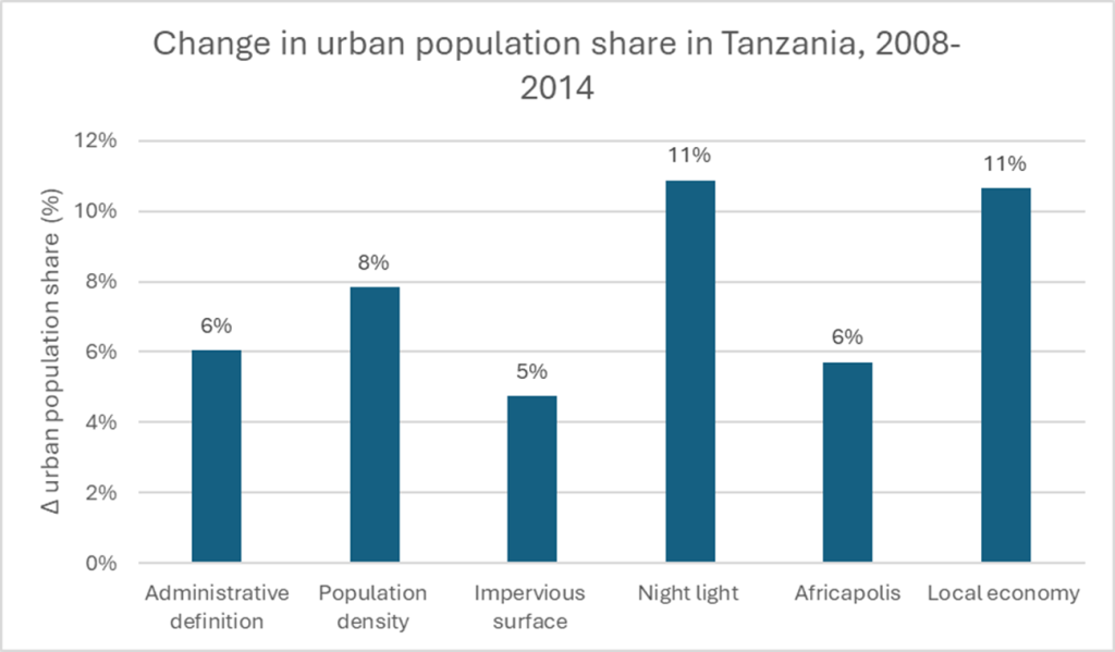
Urbanization represents a shift from a dispersed population toward one that resides in more densely populated settlements with more non-agricultural economic activities. The urbanization ‘level’ is a static point-in-time measure of the urban population share, whereas the urbanization ‘rate’ is the rate of change from a rural to urban area over time. Per official urban/rural designations, in 2014, 28% of the national population of Tanzania was urban. Between 2008 and 2014, the urbanization rate was 6%.

Using seven different definitions (Table 1), we find that urbanization levels ranged from 21% (impervious surface) to 39% (subjective assessment), and that urbanization rates over 2008-14 ranged from 6% (administrative definition) to 11% (night light and local nonfarm economy).

Figure 2: Urban population share in Tanzania, 2014. Urban population share by urban/rural definition using TZNPS LSMS-ISA household survey data.

Figure 3: Urbanization rate of change in Tanzania, 2008-2014. Urbanization rate of change by urban/rural definition using TZNPS LSMS-ISA household survey data.

Who counts as “rural” shapes what we know about rural poverty

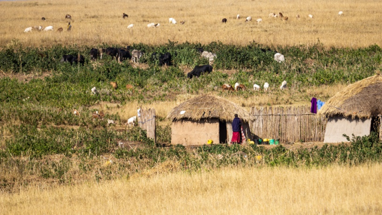
A country’s trajectory along the arc of structural transformation and poverty reduction has traditionally been tied to urbanization, and the economic orientation and rate of agricultural commercialization in rural areas. Our analyses show that the definition of “urban” can affect measures of transformation. For example, the share of the rural population with electricity is estimated to be 3% with a local economy-based definition of urban but is 9% with the night light-based definition.

To unpack this, we compared welfare characteristics of households classified as rural under both the “administrative” and “night light intensity” definitions, to those that switch from their original category with a change in definition. We find that compared to households which wererural under both definitions, those considered rural under the administrative definition but urban per the night light definition were significantly wealthier. The same applies for households considered urban under the administrative definition but rural per the night light definition. These areas that switch classification:

Have higher consumption and lower poverty rates
Spend less of their budget on food and access more of their food through purchases
Are more likely to live in homes with modern roof materials.

Lastly, we explored the income portfolios of rural households, focusing on the household’s farm income, covering the share of crop production, livestock production and agricultural wages. Across three definitions (administrative, night light, local nonfarm economy), we find that the average household income share from crops ranges from 37% – 42%, and the average income share from agricultural sources ranges from 57 – 64%. Using the administrative and night light definitions, we find that rural households are increasingly shifting away from agriculture. However, this trend is not consistent with the local economy definition, under which areas that are less agriculturally focused are recategorized to urban. Thus, “rural” appears to be static – these are, by definition, the areas that are not changing.

Periodic reclassification can create a false picture of stagnant rural welfare

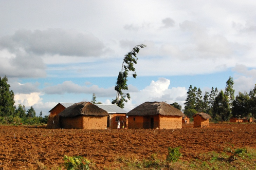
With each census, Tanzania recategorizes rural enumeration areas as urban if the town has a market, school, and/or health center and if the area essentially “feels” urban. Such a recategorization can result in rural poverty staying stagnant by definition, as successful rural areas are re-categorized as urban. Indeed, if we did not allow rural Tanzania to physically shrink over time, poverty declines slightly faster (by one percentage point), the rate of primary school completion increases faster (by one percentage point), and access to electricity increases faster (by two percentage points).

If the goal is to study transformation of the “rural” economy, care is necessary with data that crosses census reclassifications.

Lessons Learned

A 2022 UN Statistical Commission Side event announcement in 2022 noted that in addition to the centrality of urbanization in the SDG framework, it: “was also a call for collection of data at the urban level and/or disaggregation of reporting between urban and rural levels. Generation of data that is comparable at the urban level, however, requires clear definitions on what constitutes a city, as well as globally applicable metrics/ thresholds that can be applied across countries”. Until that time, large differences in official definitions of “rural”, challenge meaningful cross-country comparatives and rural time-series analyses by relegating “rural” as a residual category.

The different criteria underlying official definitions of “urban” and its residual “rural” are important to recognize when they guide country or global budget and resource allocations.

But the reality is that agreed upon and harmonized definitions may never emerge, and most official definitions are only focused on urbanization. The good news is the amount of publicly available tabular and spatial data can supplement national survey data to provide insights on specific questions, particularly those focused on changes in rural populations.

Blog written by: Samantha Petrelli, Vedavati Patwardhan and C. Leigh Anderson.

Based on: Ayala Wineman, Didier Yélognissè Alia, C. Leigh Anderson, Definitions of “rural” and “urban” and understandings of economic transformation: Evidence from Tanzania, Journal of Rural Studies, Volume 79, 2020, Pages 254-268, ISSN 0743-0167, https://doi.org/10.1016/j.jrurstud.2020.08.014. (Available here)

Additional References

Concepts, definitions and data sources for the study of urbanization: the 2030, Agenda for Sustainable Development, Eduardo López Moreno, Head Research and Capacity Development, UN-Habitat, 2017.

Patterns of household food consumption across food groups and sources in sub-Saharan African countries

Posted on November 25, 2024November 23, 2024

Background

In most low- and middle-income countries (LMICs), per capita food expenditure has been steadily rising over the past few decades despite challenges from climate change, conflict, and COVID-19. Trends in food consumption are driven by urbanization, higher incomes, globalization, increased economic integration, and consumer preferences. In sub-Saharan Africa (SSA) there has been a shift away from the consumption of staple foods toward an increasingly diversified diet. Understanding these trends, however, remains constrained by the lack of large-scale cross-national data on the pattern of consumption across a broad set of food items. In particular, there is little information on cross-country and within-country variations in food consumption patterns and how households acquire food. Agricultural livelihoods dominate most LMICs, with many households’ food consumption coming predominantly from their own production. As economies transform and agriculture transitions from subsistence to commercial farming, it is expected that households will increasingly source food from markets. Increasing consumption from locally sourced production can incentivize investment in productive farm technologies and reduce import dependency, thereby contributing to food security. In this blog, we discuss an effort led by the University of Washington Evans School of Policy Analysis and Research (EPAR) group to standardize data on the value of food consumption patterns for a large number of food items and countries in SSA. We then leverage the data to discuss some insights regarding patterns of value of food consumption by food categories, food sources, and socio-demographics.

Standardizing food consumption indicators in large-scale household survey datasets

We leverage large-scale household datasets collected by the World Bank and country National Statistical Offices to construct food consumption indicators for 16 SSA countries over the period 2008-2021. These surveys ask households to report the amount of consumption from own-production and gifts, and the amount and value of food purchased over the past 7 days prior to the interview. Consumption from purchases comprises food items that are accessed from markets. Consumption from own production refers to consumed food items that are produced by households. Consumption from gifts encompasses food items households received from other households, non-governmental organizations, and the government. The value of food consumption from own production and gift was constructed using unit values estimated in reported quantities and values of purchases. For household food item observations for which no market purchase was reported, unit prices are imputed using the median purchase price of the same food items at the lowest administrative level with at least 10 observations. Food items were aggregated into broad categories: cereals, roots and tubers, pulses, legumes and nuts, dairy, fish and seafood, fruits and vegetables, livestock products, non-dairy beverages, oils and fats, processed food, other food, meals away from home, and tobacco. For comparability across countries, the monetary value of consumption was annualized and converted to 2017 Purchasing Power Parity (PPP).

Current patterns in average total value of food consumption at the aggregate level and by food items

Figure 1 presents a graph of the average annual per capita consumption in 2017 PPP for the most recent wave of data available for included countries. Nigeria had the highest average per capita value of food consumption in 2018, while Ethiopia had the lowest average per capita value of food consumption in 2021.

Figure 2 is an interactive graph allowing a user to select one or multiple countries or years and display the average per capita value of food consumption disaggregated by food items. One takeaway is that for most countries, cereals continue to be the main food item consumed, with the highest average per capita value of consumption in all countries except Benin, Cote d’Ivoire, and Uganda. The other top food item consumed in terms of monetary value is fruits and vegetables, except in Nigeria and Uganda. The least consumed food items are pulses and legumes and roots and tubers, with the exception of Uganda where oils/fats and non-dairy beverages are the least consumed food items. For countries with multiple years of data, we can examine trends in the per capita value of food consumption over time. We see, for example, a consistent increase in the value of consumption of cereals, pulses, legumes and nuts in Malawi and Mali.

Patterns in the value of food consumption by sources

Figure 3 presents the average annual share of the value of household food consumption from purchases, own production, and gifts. Across all countries and years, about 75% of household value of food consumption is from market purchases, while own production and gifts represent 20% and 5% respectively. There are substantial variations across countries and over time. Senegal had about 93% of its household value of food consumption acquired through purchases in 2018 while the lowest share was recorded in Uganda in 2011 (46%). For most countries, the relative importance of market-sourced food is growing. For example, in Uganda, the share of food from markets increased from, 46% in 2011 to 59% in 2019. Similar growth was observed in Ethiopia, Tanzania, and Niger.

Figure 4 presents an interactive graph showing the average share of the value of household food consumption from purchases, own production, and gifts, disaggregated by major food categories. It reveals that for most food categories, more than 60% of consumption comes from purchases. This is particularly true for high-value commodities such as fish and seafood, livestock products, fruits and vegetables, oils and fats, non-dairy beverages, and processed food. For staple crops such as cereals, pulses, and roots and tubers, the purchased share is lower. The consistency of shares by sources over time also varies; for example, Tanzania consistently had more than 50% of its dairy consumption from own production while in Malawi, less than 20% of dairy consumption come from own production. We see a gradual decrease in consumption of pulses, legumes, and nuts from own-production and a resulting increase in consumption from purchases and gifts. The share of roots and tubers increased for most of the waves in Tanzania while there was a consistent decrease in Nigeria.

Spatial and gender heterogeneity in the value of household food consumption

Figure 5 presents an interactive spatial distribution of the total value of food consumption from purchases, own production, and gifts at both country and administration one levels. The maps can be further disaggregated by year, location, and gender of household head. These maps show that countries in East Africa had a greater value of food consumption from their own production compared to other SSA countries. The estimates mapped can also be disaggregated by place of residence and the gender of the head of household to produce location- and gender-specific insights. This insight holds for both male and female-headed households as well as households located in both rural and urban areas. This distinction is further strengthened when consumption is disaggregated by food items (see Figure 7).

Figure 6 explores differences in the share of the value of food consumption from different sources disaggregated by location. On average across countries, about 65% of food consumption for rural households comes from purchase. This percentage rises to about 90% for urban households in most countries, except Kenya and Uganda.

Figure 7 presents the same interactive graph as Figure 6 but is further disaggregated by the gender of the household head. Here, we see that for most countries, female-headed households (FHHs) residing in urban areas have a higher share of food consumption value from purchases compared to their counterparts in rural areas. The same distinction is also applicable for male-headed households (MHHs). The reverse is the case in Malawi where FHHs in both urban and rural areas have a lower share of food consumption value from purchases compared to MHHs. More generally, MHHs in both urban and rural areas tend to have a higher share of food consumption value from own production compared to FHHs.

Concluding remarks

This blog provides insights into the sources and patterns of the value of food consumption in SSA. It leverages a new dataset put together by EPAR processing and merging food consumption indicators in nationally representative large-scale household surveys collected in 16 SSA countries over the period 2008 – 2021. The analysis reveals that of the different sources of food examined, market-purchased consumption accounts for the highest value, even in rural areas. It also shows a rapid shift towards increased value of food consumption from purchases, marking a departure from traditional practices of consuming own-produced food and gifts. The analysis indicates that this shift is not uniform across countries and socio-demographic characteristics of households within countries. These shifts, rooted in socio-economic changes, gender roles, and urbanization, underscore the complex challenges and dynamics facing global food security and nutrition strategies. The dataset can be used to help understand changes in food sourcing and what this might mean for nutrition, resilience, and market access. The Stata codes to generate the dataset is available for download at the EPAR GitHub Repository. The more complete visualization data is also accessible on tableau visualization platform.

Blog written by Amaka Nnaji, Ahana Raina, Didier Alia and C. Leigh Anderson.